Geographies in the Census Geocoder¶

Introduction
Benchmarks, Vintages, and Layers
- Benchmarks and Vintages
- Layers
Census Geographic Hierarchies Explained

Introduction ¶

We like to think that geography is simple. There’s a place, and that place has some borders, and it’s all easy to understand. Intuitive, right?

Wrong.

Geography is actually extremely complicated, because it is by its very nature ambiguous. The only objectively unambiguous definition of a geographic area is a pair of longitude/latitude coordinates. When you start considering ways in which geographic areas overlap or roll into a hierarchy, it gets even more complicated because then you need to consider how each geographic area gets defined and overlaps.

Then, when you consider how such geographic hierarchies map to data (which itself represents a point-in-time), it gets even more complicated. That’s because geographic definitions change all the time. Street names change, town names change, borders shift, etc.

And the Census Geocoder API and the US Census Bureau data that it corresponds to has to inherently account for all of these complexities. Which makes the way the Census Geocoder API handles geographic areas complicated.

Benchmarks, Vintages, and Layers ¶

Benchmarks and Vintages ¶

The data returned by the Census Geocoder API is different from typical geocoding services, in that it is time-sensitive. A geocoding service like the Google Maps API or Here.com only cares about the current location. But the US Census Bureau’s information is inherently linked to the statistical data collected by the US Census Bureau at particular moments in time.

Thus, when making requests against the Census Geocoder API you are always asking for geographic location data or geographic area data as of a particular date. You might think “geographies don’t change”, but in actuality they are constantly evolving. Congressional districts, school districts, town lines, county lines, street names, house numbers, etc. are all constantly evolving. And to ensure that the statistical data is tied to the locations properly, that alignment needs to be maintained through two key concepts:

Benchmarks

Vintages

The benchmark is the time period when geographic information was snapshotted for use / publication in the Census Geocoder API. This is typically done twice per year, and represents the “geographic definitions as of the time period indicated by the benchmark”.

The vintage is the census or survey data that the geographies are linked to. Thus, the geographic identifiers or statistical data associated with locations or geographic areas within a given benchmark are also linked to a particular vintage of census/survey data. Trying to use those identifiers or statistical data with a different vintage of data may produce inaccurate results.

The Census Geocoder API supports a variety of benchmarks and vintages, and they are unfortunately poorly documented and difficult to interpret. Therefore, the Census Geocoder has been designed to streamline and simplify their usage.

Vintages are only available for a given benchmark. The table below provides guidance on the vintages and benchmarks supported by the Census Geocoder:

	BENCHMARKS
	Current	Census2020
VINTAGES	Current	Census2020
	Census2020	Census2010
	ACS2019
	ACS2018
	ACS2017
	Census2010

When using the Census Geocoder, you can supply the benchmark and vintage directly when executing your geocoding request:

import census_geocoder as geocoder

result = geocoder.location.from_address('4600 Silver Hill Rd, Washington, DC 20233',
                                        benchmark = 'Current',
                                        vintage = 'ACS2019')

result = geocoder.geography.from_address('4600 Silver Hill Rd, Washington, DC 20233',
                                         benchmark = 'Current',
                                         vintage = 'ACS2019')

See also

import census_geocoder as geocoder

result = geocoder.location.from_address(street = '4600 Silver Hill Rd',
                                        city = 'Washington',
                                        state = 'DC',
                                        zip_code = '20233',
                                        benchmark = 'Current',
                                        vintage = 'ACS2019')

result = geocoder.geography.from_address(street = '4600 Silver Hill Rd',
                                         city = 'Washington',
                                         state = 'DC',
                                         zip_code = '20233',
                                         benchmark = 'Current',
                                         vintage = 'ACS2019')

See also

import census_geocoder as geocoder

result = geocoder.location.from_coordinates(longitude = -76.92744,
                                            latitude = 38.845985,
                                            benchmark = 'Current',
                                            vintage = 'ACS2019')

result = geocoder.geography.from_coordinates(longitude = -76.92744,
                                             latitude = 38.845985,
                                             benchmark = 'Current',
                                             vintage = 'ACS2019')

See also

import census_geocoder as geocoder

result = geocoder.location.from_batch(file_ = '/my-csv-file.csv',
                                      benchmark = 'Current',
                                      vintage = 'ACS2019')

result = geocoder.geography.from_batch(file_ = '/my-csv-file.csv',
                                       benchmark = 'Current',
                                       vintage = 'ACS2019')

See also

Hint

Several important things to be aware of when it comes to benchmarks and vintages in the Census Geocoder library:

Unless over-ridden by the CENSUS_GEOCODER_BENCHMARK or CENSUS_GEOCODER_VINTAGE environment variables, the benchmark and vintage default to 'Current' and 'Current' respectively.

The benchmark and vintage are case-insensitive. This means that you can supply 'Current', 'CURRENT', or 'current' and it will all work the same.

If you want to set a different default benchmark or vintage, you can do so by setting CENSUS_GEOCODER_BENCHMARK and CENSUS_GEOCODER_VINTAGE environment variables to the defaults you want to use.

Layers ¶

When working with the Census Geocoder API (particularly when getting geographic area data), you have the ability to control which types of geographic area get returned. These types of geographic area are called “layers”.

An example of two different “layers” might be “State” and “County”. These are two different types of geographic area, one of which (County) may be encompassed by the other (State). In general, geographic areas within the same layer cannot and do not overlap. However different layers can and do overlap, where one layer (State) may contain multiple other layers (Counties), or one layer (Metropolitan Statistical Areas) may partially overlap multiple entities within a different layer (States).

When using the Census Geocoder you can easily specify the layers of data that you want returned. Unless overridden by the CENSUS_GEOCODER_LAYERS environment variable, the layers returned will always default to 'all'.

Which layers are available is ultimately determined by the vintage of the data you are retrieving. The following represents the list of layers available in each vintage:

Note

You may notice that there are (logical) duplicate layers in the lists above, for example “2010 Census PUMAs” and “2010 Census Public Use Microdata Areas”. This is because there are multiple ways that users of Census data may refer to particular layers in their work. This duplication is purely for the convenience of Census Geocoder users, since the Census Geocoder API actually uses numerical identifiers for the layers returned.

When geocoding data, you can simply supply the layers you want using the layers keyword argument as below:

import census_geocoder as geocoder

result = geocoder.location.from_address('4600 Silver Hill Rd, Washington, DC 20233',
                                        benchmark = 'Current',
                                        vintage = 'ACS2019',
                                        layers = 'Census Tracts, States, CDPs, Divisions')

result = geocoder.geography.from_address('4600 Silver Hill Rd, Washington, DC 20233',
                                         benchmark = 'Current',
                                         vintage = 'ACS2019',
                                         layers = 'Census Tracts, States, CDPs, Divisions')

See also

import census_geocoder as geocoder

result = geocoder.location.from_address(street = '4600 Silver Hill Rd',
                                        city = 'Washington',
                                        state = 'DC',
                                        zip_code = '20233',
                                        benchmark = 'Current',
                                        vintage = 'ACS2019',
                                        layers = 'Census Tracts, States, CDPs, Divisions')

result = geocoder.geography.from_address(street = '4600 Silver Hill Rd',
                                         city = 'Washington',
                                         state = 'DC',
                                         zip_code = '20233',
                                         benchmark = 'Current',
                                         vintage = 'ACS2019',
                                         layers = 'Census Tracts, States, CDPs, Divisions')

See also

import census_geocoder as geocoder

result = geocoder.location.from_coordinates(longitude = -76.92744,
                                            latitude = 38.845985,
                                            benchmark = 'Current',
                                            vintage = 'ACS2019',
                                            layers = 'Census Tracts, States, CDPs, Divisions')

result = geocoder.geography.from_coordinates(longitude = -76.92744,
                                             latitude = 38.845985,
                                             benchmark = 'Current',
                                             vintage = 'ACS2019',
                                             layers = 'Census Tracts, States, CDPs, Divisions')

See also

import census_geocoder as geocoder

result = geocoder.location.from_batch(file_ = '/my-csv-file.csv',
                                      benchmark = 'Current',
                                      vintage = 'ACS2019')

result = geocoder.geography.from_batch(file_ = '/my-csv-file.csv',
                                       benchmark = 'Current',
                                       vintage = 'ACS2019',
                                       layers = 'Census Tracts, States, CDPs, Divisions')

See also

Hint

When using the Census Geocoder to return geographic area data, you can request multiple layers worth of data by passing them in a comma-delimited string. This will return separate data for each layer indicated. The comma-delimited string can include white-space for easy readability, which means that the following two values are considered identical:

layers = 'Census Tracts, States, CDPs, Divisions'

layers = 'Census Tracts,States,CDPs,Divisions'

To retrieve all available layers that have data for a given location, you can submit 'all'. Unless you have set the CENSUS_GEOCODER_LAYERS environment variable to a different value, 'all' is the default set of layers that will be returned.

Note that layer names in the Census Geocoder are case-insensitive.

Census Geographic Hierarchies Explained ¶

As you can tell from the list of layers above, there are lots of different types of geographic areas supported by the Census Geocoder API. These areas overlap in lots of different ways, and the US Census Bureau’s documentation explaining this can be a little hard to find. Therefore, I’ve tried to explain the hierarchies’ logic in straightforward language and diagrams below.

See also

Core Hierarchy ¶

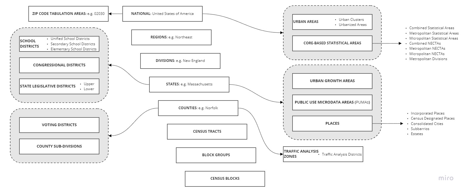
We should start by understanding the “core” of the US Census Bureau’s hierarchy, and working our way “up” from the smallest section. This core hierarchy by definition does not overlap. Each area within a particular level of the hierarchy is precisely defined, with those definitions represented in the Tigerline / Shapefile data published by the US Census Bureau.

Census Block: The single smallest element in the core hierarchy is the Census Block. This is the most granular geographical area for which the US Census Bureau reports data, and is the smallest geographic unit where data is available for 100% of its resident population.

Block Groups

Collections of Census Blocks. In general, the population size for block groups are 600 - 3,000.

This is the most granular geographical area for which the US Census Bureau reports sampled data.

Census Tracts

Collections of Block Groups. They are considered small, permanent, and consistent statistical sections of their containing county.

Optimally contains 4,000 people, and range from 1,200 - 8,000 people.

Counties and County Equivalents

The first administrative (government administered) area defined in the core hierarchy. Counties have their own administrations, subordinate to the state administration. Defined as a collection of Census Tracts.

Note

In 48 states, “counties” in the data correspond to “counties” in the their legal administration.

In MD, MO, NV, and VA, Independent Cities are treated as counties.

In LA, parishes are treated as counties.

In Alaska, Cities, Boroughs, Municipalities, and Census Areas are treated as counties.

In Puerto Rico, municipios are treated as counties.

In American Samoa, islands and districts are treated as counties.

In the Northern Marianas, municipalities are treated as counties.

In the Virgin Islands, islands are treated as counties.

Guam and the District of Columbia are each treated as a county.

In addition to breaking down into census tracts, counties may also be broken down into:

County Subdivisions
Voting Districts

States¶

The federally-constituted state (or territory, as applicable). Defined as a collection of Counties.

In addition to breaking down into counties, states may also be broken down into:

School Districts
Congressional Districts
State Legislative Districts

States also include Places, which are named entities in several types:

Incorporated Places. Which are legally-bounded entities with some form of local governance recognized by the state. Typically they are referred to as cities, boroughs, towns, or villages.

Census Designated Places. Which are statistical agglomerations of unincorporated areas that are still identifiable by name.

Consolidated Cities. Which are statistical agglomerations of city-related places.

Divisions¶: Collections of states that comprise a division within the USGIS definition of divisions.

Regions¶: Collection of divisions that comprise a region, per the USGIS definition.

National¶

Collection of all regions, that in total makes up the United States of America.

In addition to breaking down into regions, the country can also be broken down into:

Zip Code Tabulation Areas

Hint

It may be surprising that zip code tabulation areas are not defined at the state level. There are several important reasons for this fact:

First, ZCTAs in the Census definition are only approximate matches for the US Postal Service’s zip code definitions. They are statistical entities that are composed of Census Blocks, and so may not align perfectly to building zip codes.
Zip codes in general are federally administered by the US Postal Service, and in some (very rare!) cases zip codes may actually straddle state lines.

The country also contains a number of standalone geographical areas, which while not comprising 100% of the nation, may represent significant sections of the country or its component parts. In particular, the country also includes:

Core-based Statistical Areas. These are statistical areas that are composed of census blocks and which are used to represent different population agglomerations. Examples include Metropolitan Statistical Areas (which are statistical agglomerations for a given metro area), or NECTAs (New England City and Town Areas, which are division-specific agglomerations of New England communities).
Urban Areas. These are statistical areas that are composed of census blocks, and which have two types: urban clusters (which contain 2,500 - 50,000 people) and urbanized areas (which contain 50,000 or more people).

Secondary Hierarchies ¶

Budding off from the core hierarchy, specific geographic entities can either be broken down or contain other secondary hierarchies. Most secondary hierarchies are flat (i.e. they are themselves defined by a collection of census blocks), but they may be composed of different types of entities.

A good example of this pattern is the secondary-hierarchy concept of “School District”. While school districts cannot be broken down further (they are defined by census blocks), there are three types of school district that are available within the US Census data: Unified School Districts, Secondary School Districts, and Elementary School Districts.

Places ¶

Another major secondary hierarchy with similar “type-based” differentiation is the concept of “places”. There are multiple types of place, including Census Designated Places, Incorporated Places, and Consolidated Cities. These are conceptual areas, which in turn can all be broken down into their component census blocks.

The most important types of places are:

Incorporated Places. Which are legally-bounded entities with some form of local governance recognized by the state. Typically they are referred to as cities, boroughs, towns, or villages.

Census Designated Places. Which are statistical agglomerations of unincorporated areas that are still identifiable by name.

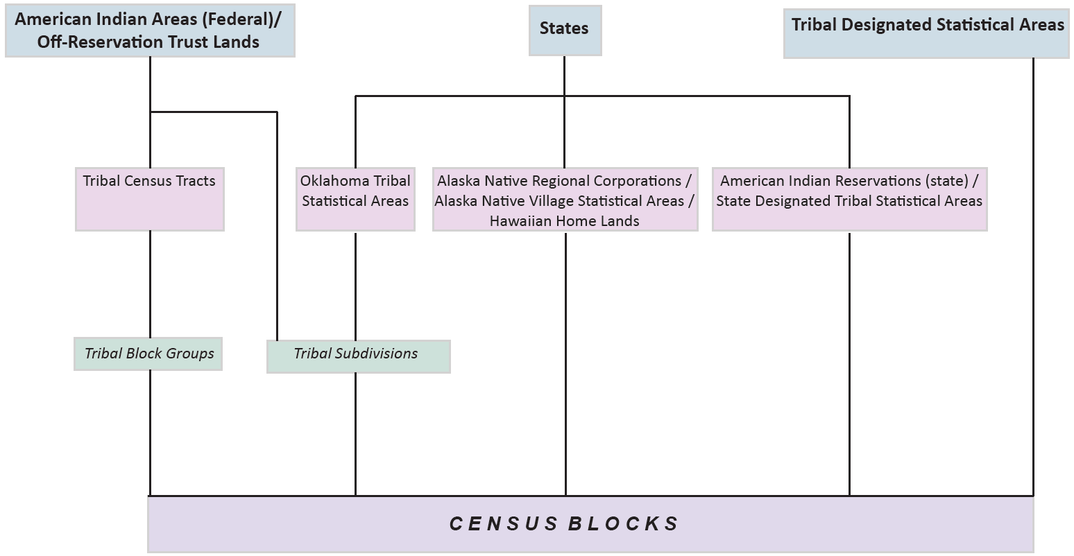
AIANHH Hierarchy ¶

Besides the core hierarchy described above, the US Census Bureau also reports data within an American Indian, Alaska Native, and Native Hawaiaan-oriented hierarchy.

This hierarchy is also built by rolling-up Census Blocks, however it does not conform to either the state or county-level definitions used in the core hierarchy. This is because tribal population groups, federally-designated American Indian areas, tribal-designated areas, etc. may often cross state, division, or regional lines.

American Indian, Alaska Native, and Native Hawaiian Hierarchy